ArcPad Data Collection

Introduction

            Our final exercise of the semester involved creating a database in ArcPad for deployment in the field.  Using the ArcPad software, we were able to create pre-designated data fields and import them onto a Juno GPS.  Creating a database prior to gathering data in the field, allows the user to limit his/her input, therefore reducing the potential for error. This practice should be considered standard procedure when embarking in any geospatial field activity.

Study Area

            The study area for this exercise was once again the 112 acre plot of land known as the Priory (figure 1).

Figure 1. Priory study area located south of UWEC Campus 

 

Methods

            We began this activity by creating a geodatabase within ArcMap including our three desired fields, benches, erosion, and invasive species. For each of the fields we created a domain to describe attributes of the data being collected.  For example, benches may fall under one of three values, usable, needs repair, and unusable.  A description is provided with each of the values to define our interpretation of the feature.  In the case of erosion, a coded value signifying severe levels of erosion would describe that feature as having exposed bedrock, outcropping, wasting, or colluvium debris.

            After the database has been created, a project was made within ArcMap. It was important to classify the three fields using a distinct symbol that can be recognized in the field. A projected raster background image was also included in the project to spot our visual location on the GPS unit. Using the ArcPad Data Manager, we prepared our database to be imported as an ArcPad project. Once this was complete, we were able to transfer our ArcPad map (.apm) file onto the the GPS device.  We used the Juno 3B Trimble model for field data collection (figure 2).



Figure 2: The Juno 3B Trimble GPS unit used during the data collection portion of this activity

 

            Once all of the data is transferred to the Juno, we were able to collect our points in the field.  The intuitive design of the Juno allows the user to simply select the feature being recorded, and the location data is automatically stored for the previously defined projection. When selecting the feature, the display will ask how to classify it according to the set domain.  After marking the features, the unit automatically saves them to your .apm file and they are ready to be uploaded.

            Uploading the data is quite easy. Simply use the ArcPad Data Manage and select ‘get from ArcPad’. The software wizard will prompt you to select your file and it will then upload the data. The map I created below shows where each feature is located as well as its condition (figure 3).

Figure 3: The point locations of the three feature, benches (star), erosion (diamond), and Buckthorn (bolt).

Conclusion

            Although we only used a week to cover this lesson, I can see its potential in creating an organized and thorough database.  It’s important to begin any field activity from the ground up instead of collecting data on the fly.  This procedure will help organize your data from the get go while reducing the amount of error that may occur during the data collection phase of the project. I look forward to getting more hands on experience with ArcPad and the Juno devices in future projects.

 

High Altitude Balloon Launch

On April 26, 2013, geography 336 students launched their high altitude balloon equipped with a Flip video camera and a GPS tracker.  The balloon reached 100,000 feet before bursting and parachuting to the ground.  Using the GPS tracker, the balloon was recovered nearly 80 miles west of the launch site in Marshfield Wisconsin. The video below is an edited version of the HABL flight.

Balloon Mapping Part 1

Introduction:

Often times the quality of aerial imagery attained is limited by funding.  In this lab, we used a low cost weather balloon and a digital camera to create high resolution imagery of the University of Wisconsin Eau Claire campus.  Although the weather conditions were far from ideal, we were able to capture multiple images suitable for mosaicking within the ArcMap software to create one seamless map. What we learned throughout this lab will also be used in subsequent labs to increase the quality of our aerial maps.

Methods:

Two cameras were being used throughout the mapping process, one a Lumix digital camera, the other a Flip video recorder.  The digital camera was set on landscape mode for better focus quality and used continuous shot to capture multiple images while in flight.  The Flip video camera was used to test the upcoming high altitude balloon launch.

Both cameras were housed within a small Styrofoam box, commonly used as a fishing worm container.  A hole with the diameter of each camera lens was cut into the Styrofoam box to capture the entire scene below.  The Flip camera also used Velcro to secure it in position, and a small GPS tracker was also enclosed within the box to test a payload similar to what will be seen in the high altitude launch.  The only other equipment used during this launch was a etrex GPS unit.  The GPS unit is being used to record coordinates that will be used when georeferencing and mosaicking the images.

To fill the balloon, we transported a large helium tank to our storage facility, attached a rubber hose to the regulator and began filling the balloon.  To avoid puncture, at least three colleagues held the balloon secure at all times.  A thin piece of rope was also fastened to the end of the balloon and used as a carry handle.  Once the balloon was filled, zip ties were used to close its end around the plastic ring where the payload box and control string were attached. 

To attach the payload box, 550 cord was wrapped and secured around all four sides of the box.  The 550 cord was tied into a knot, ensuring all four sides were equal in length.   A carabineer was clipped through the knot and attached to the filled balloon.

Figure 1: Rope harness holding the payload box flat (hopefully)

Figure 2: Adding the payload box to the balloon.

A thin nylon string measured and marked at 50 foot increments was used to control the balloons flight path and altitude.  Once 400 feet of string was measured and marked, we used another small carabineer to attach it to the balloon. 

Figure 3: Measuring 400' of control string at 50' increments

Our setup now being complete, we prepared for the launch.  The digital camera box was the first being deployed.  After turning on the camera and activating landscape and continuous shot mode, we began unrolling the balloon slowly to 400 feet.  Everything went according to plan except one major factor.

Results:

The weather on the day of our launch was far from ideal.  A strong crosswind prevented the balloon from reaching the designated elevation of 400 feet above ground.  Strong gusts caused unpredictable flight characteristics creating many oblique images to varying degrees.  Although most of the images were largely oblique, there were enough suitable ones to mosaic together. 

Figure 4: A strong crosswind caused most of the captured photos to be oblique images.

 

After we pulled in the Lumix camera, the Flip box was clipped on as a HABL test. It had similar flight characteristics as the digital camera, however, our control string broke under the tension.  Although we lost our balloon, the payload box was salvaged as it fell into the Chippewa River.

After importing the select few suitable photos into ArcMap, I used a projected aerial image file to begin georeferencing.  A minimum of nine control points were used on each one of the photos.  After georeferencing one photo, I used control points on it for the next.  I figured this process would reduce a visible seam as much as possible.  Although seams are still present, the mosaicked image is much better than what I had expected.

Conclusion:

This exercise was a great learning process for future launches.  Weather considerations will be even more important when the time comes for our high altitude launch.  Although the quality of the mosaic wasn’t the greatest, it let us know what needs to be improved on in future launches. 

 

Final Land Navigation

Introduction:

This week’s activity brought an end to our land navigation exercises. We were tasked with using everything we learned thus far in a game of paintball at the Priory land. By applying a culmination of skills learned in previous weeks, we were required to locate and navigate to the points throughout the course in the most efficient manner possible.  We used the week to create new maps, including the point locations and off limit boundaries, as well as develop a strategy for our team’s success.  Each of the six teams were able to determine their own course of action, making encounters very likely.  This exercise provided a fun activity in which we could hone our skills and show what we learned throughout the land navigation section of our geospatial field methods class.

Study Area:

Once again the study area for this week’s activity was the 112 sq acre Priory land purchased by the University of Wisconsin Eau Claire in October of 2011. Figure 1 below shows the location of the Priory from the UWEC campus. Having already navigated this course, we were familiar with the terrain making it much easier to establish a sense of direction.

 

Methods:

During week 1 of our land navigation project, we began preparations for compass/map navigation.  This traditional method provides an effective means of travel without the reliance on technologies such as the global positioning system (GPS).  The only elements required for this technique are distance and direction. The use of a compass and a map provide you with the needed information to determine direction, while a 100 meter pace count offers you the element of distance.

We began by establishing our pace count using the TruPulse range finder, used in our distance azimuth survey, to measure 100 meters.  After measuring 100 meters, determining your pace count is as simple as counting every other step from start to finish.  My recorded pace count ended up being 65 steps; however, since this was a straight line path, on concrete, I decided to add 10 paces to account for being in the woods and traveling in a less linear path. Using the scale included on my maps, I can measure the map distance between each point and associate it with my pace count to determine my ground distance.

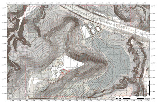
The second portion of land navigation week one, involved using ArcMap to create the maps used during the exercise.  The only requirement for these maps was that they use a UTM grid reference system.  Since the points are being provided to us in UTM, we have to use the same grid system to determine their location.  I decided on using two maps, one with very detailed contour lines to easily distinguish changes in relief (figure 2), and the other showing a clear aerial photograph to distinguish changes in vegetation (figure 3).  As you can see in figure 2, the major terrain features are made visible using 2 foot contour intervals. Figure 3 shows the contrast between the different vegetation quite clearly.  For both maps, 50 square feet grid intervals were used to keep them cluster free while plotting the points.

During the second week of the land navigation activity, we put our maps and pace counts to use using a traditional map and compass technique. Traditional land navigation not only retracts from our reliance upon technology that often fails, it also provides an accurate and efficient means of travel.

The first part of compass/map navigation is plotting the coordinates of the course’s points.  These points were given to us in six digit UTM coordinates, making them accurate to within 10 meters of the point’s actual coordinates. Using the grid references on our map, made this process as simple as aligning the first three digits with the x-axis and the last three digits with the y-axis. Figure 4 shows our point locations marked on our map, point 1B being the starting point.

After plotting the coordinates, we determined the direction of travel by finding the azimuths. An azimuth is simply the straight line direction between two points with units in degrees or mils. The technique I used involved placing a military protractor on each point and aligning its crosshairs parallel to the grid lines. A straight edge can then be used to record the direction in degrees found on the outside edge of the protractor (Figure 5).

The last preliminary step before starting the course is to use the map’s scale to determine the distances between each point. This distance in meters can then be converted into your pace count so that your location on the map is known.

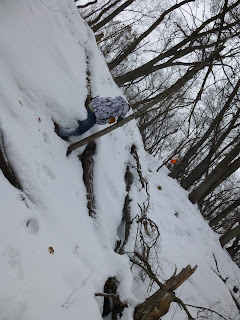
After all of the points were plotted, the direction of travel determined, and distances measured, we moved to our first course marker.  We began at the starting location and pointed our compass to our first azimuth towards point 2B. Once each point was found, we simply rotated the bezel on our compass to align it with the next azimuth. Using this simple, traditional technique, was quite efficient in finding all six of our points. The most difficult part of the process was walking in snow at times being two feet deep (Figure 6).  

Land navigation part three involved using a global positioning system to find a different set of points on the Priory course. This technique provided some advantages and disadvantages for finding our points.  The advantages being that it allows us to track our movement throughout the course using the track log feature, and it makes having a map less necessary since it provides your locations coordinates.  However, using a GPS also has disadvantages such as reliance on batteries, it being subject to a harsh environment, and strength of signal in dense vegetation.

For our GPS land navigation exercise, we used a Garmin etrex GPS unit. Although somewhat outdated, this unit is relatively inexpensive and useful for simple tasks such as land navigation.  By using at least three satellites, a GPS triangulates your location on a three dimensional plane in X, Y, and Z fields. This provides good locational data to be incorporated within a GIS.  After being given our point coordinates, we activated the GPS track log and moved towards the first point. Using the X and Y coordinates displayed on the GPS, we walked towards our point coordinates. This technique was very slow, as we often found ourselves walking out of our way to determine which direction we needed to go. 

Once the course’s points were found, we were able to upload our track log data to see our route. Figure 7 shows my groups track log as we navigated our course.  Right off the bat you can see our direction got mixed up in the south west area near the parking lot.

After each group uploaded their track logs, I imported the data into ArcMap. In figure 8 you can see that all 18 of the points were reached. By incorporating the time data stored by the GPS, you can see which groups were more efficient in their travel (Figure 9).

FIGURE 9 GROUPS ANIMATION

Results:

Having learned the necessary skills for both traditional and GPS land navigation, our final test was to travel to as many points as possible with the added element of paintball.  Using our experience in the previous weeks, we recreated our maps showing off limits zones and the necessary information ensuring our success. 

Once again, we used our GPS’s track log feature to record our routes; however, already being familiarized with the course, we relied much more on terrain association than the actual GPS coordinates. This provided a very efficient way of reaching the points, while staying alert for the five other groups.  In figure 10, you can see our route, along with the other groups. Our routes meeting were often accompanied by an intense firefight and a hasty retreat by one team or the other.

 

To accompany this data, I created a time animation showing each groups travel throughout the course.  Figure 11 clearly shows where groups converge on one another and a firefight occurs.

FIGURE 11 CLASS TRACKLOG TIME ANIMATION

Conclusion:

Using the methods learned throughout the land navigation portion of our class, I feel quite confident in my abilities to find feature locations using either, a compass and a map, or a global positioning system.  These skills can be used for various field activities conducted by geographers, such as collecting feature data on a study area.

GPS Navigation

Introduction:

As an extension of last week’s activity, this week we navigated the Priory course using a global positioning system.  Features within the GPS allowed us to track and upload our paths to the various points making it effective in showing our precise locations.   This relatively modern technique has a number of advantages and disadvantages that will be covered in the course of this report.

Study Area:

Methods:

For our GPS land navigation exercise we used a Garmin etrex GPS unit (figure 1).  Although this unit is somewhat outdated compared to a more modern GPS, they are quite inexpensive and useful for simple tasks such as land navigation.  By using at least three satellites this system can determine your location on an X, Y, and Z axis.  Once the GPS location is triangulated using the satellites, the location can be displayed either as coordinates or with a map marker.  For our purposes, we used the coordinates displayed using a UTM coordinate system. 



Figure 1: The Garmin etrex GPS was used throughout the data collection process. Data points were collected using the track log feature and uploaded into ArcMap to view spatially.

After being given our point locations and our punch card, our group activated the GPS track log and set off towards the first point.  The track log is simply a saved coordinate location using a set time interval.  This feature will be explained further in the results portion of this report.  For finding our points we used the simple technique of watching our X and Y coordinates increase or decrease in the direction of our point.  This procedure became quite painful as we navigated in steep, snow covered terrain trying to find the correct direction.  Figure 2 shows the conditions we had to traverse through.

Figure 2: The conditions were far from ideal with snow drifts up to two feet deep.  Navigating through this much snow was exhausting but fun.

Snow picture

After finding all of our points, we were tasked with uploading our track log data and dismissed from class.  The track log data was quite easy to upload using the DNR GPS program provided on University computers.  Once the GPS is plugged in with a USB cord you can connect to it by selecting Connect to Default GPS located in the GPS tab (figure 3).



Figure 3: For the DNR GPS program to recognize the GPS, you must first establish a connection.

Once the GPS device is recognized you can begin adding your track log by selecting download under the Track tab (figure 4).  The program will then begin extracting your data to the computer for you to save.  It may take a few minutes depending on the amount of points that were stored on the GPS.  Some people had relatively fewer points than others, for example my GPS stored 5,795 points while Joey’s only stored 576.

Figure 4: Once the GPS is connected to the program, you can begin downloading your data points. The image above shows the location for downloading your log.

After the points are all uploaded onto the computer, the next step is to save them as a shapefile to be imported and projected using ArcMap.  To save the points as a shapefile navigate to file>save to> arcMap>file. Next you will be prompted to name your file and select the file type important: make sure you select ESRI Shapefile (*.shp) as the type as seen in figure 5.

Figure 5: It is important so save your data as a shapefile so that it can be easily uploaded into ArcMap.  Once the data was in ArcMap, we saved it as a feature class for ease of distribution.

The data is now ready to be imported into arcMap and saved as a feature class to be distributed amongst our group. Figure 6 shows my uploaded track log in ArcMap.

Figure 6: My uploaded track log showing where I traveled throughout the Priory.

Results:

After conducting this navigation exercise, I prefer using the traditional map and compass technique.  It seemed that the GPS technique was much less efficient. We spent a lot of our time walking in one direction just to find our numbers getting further away from our goal and then having to backtrack. Figure 7 below shows my track log projected on an aerial image of the study area.  Notice the southwest group of points and how many directions we traveled just to orient ourselves towards the first point.  After finding point 1, we started to get the hang of it a little better; however, we still found ourselves straying at times and needed to correct our direction. We would have found the points much more quickly had we set a waypoint to the coordinates given.

Figure 7: After exporting my shapefile as a feature class, I was able to give it the same projection as the Priory aerial image. I could then add the layers I felt appropriate for showing my navigation. Using this map you can tell which points my group was tasked with finding.

For the most part, our group’s track logs all lined up with one another’s. In certain cases, we would send someone in one direction and another person in a different direction to compare the coordinates.  Many of the curves seen in the track logs, such as east of point 3a, are caused by us maneuvering around obstacles like steep draws (figure 8).

Figure 8: Showing the routes taken by group 6. Most of the points match up fairly well. Locations where the points deviate from one another are caused by the technique of sending two members in different paths to compare coordinates.

The classes track log data shows all of the points being visited by each group.  Groups that inserted the coordinates as a waypoint were much more efficient on reaching their points in a timely manner. Figure 9 shows each person navigating throughout the course.

Figure 9: All 18 points were visited by at least one group. 

Conclusion:

Despite the difficult terrain and heavy accumulation of snow, our group was able to navigate to all of our points.  Although I felt the GPS technique was less efficient than traditional map and compass navigation, it gave us lots of data to incorporate into a geographic information system.  In the upcoming post, I will be using time animation to provide additional information on our activity.

Traditional Land Navigation

Introduction:

On Monday March 5^th we conducted our first land navigation field activity using traditional methods.  The only tools needed for this technique were our maps created during last week’s activity and an orienteering compass.  Although this technique is considered archaic when used alongside new age technology, it is highly reliable and if done correctly very accurate.  Land navigation with a compass and map is to this day still a fundamental skill used by our Armed Forces.  During times when your Blue Force Tracker or Dagger GPS malfunction, the next reliable alternative is compass/map navigation.

Methods:

Having already created our maps and recorded our pace counts, the next process in this exercise was to plot our points.  The points were given to us in 6 digits for both the X and Y coordinates making it very easy for us to use our UTM reference grids.  Once the general area within our 20X20 meter grid cells was located, we could easily interpolate an even more accurate location of the point.  Figure 1 below shows all six of the points plotted on our aerial image map.  Point 1B was our starting location just outside the Priory building.  After we all plotted our points individually on separate maps, we were able to compare them with each other to minimize error in plotting.  

Figure 1: Our map after plotting the 6 points. Point 1B on this map was moved slightly to the north after this image was taken.

After plotting, we determined the azimuths connecting all six of our points.  An azimuth is simply the straight line direction between two points with units of degrees or mils. The technique I used involved a military protractor.  Figure 2 shows me finding the azimuth between two points.  Using the protractor, you simply place the middle crosshair on your point and parallel to the grids. Next, use a straight edge to record the direction in degrees found on the outside edge of the protractor. 

Figure 2: This image shows me finding the azimuths to each of our points using a military protractor. If you look closely you can see a small nylon string going through the center of the protractor. This string is used for on the fly azimuth calculations without having to draw a line between your points or use a straight edge (as shown in this photo).

Another method of determining an azimuth is by using your compass.  Figure 3 is an orienteering compass like what was provided to us.  To find an azimuth simply place the compass on your map and use the straight edge of the base plate with the direction of travel arrow towards your point. Next twist the bezel with index lines so that North is oriented to North on your map and the index lines are parallel to your grid lines.  To find your azimuth, turn the compass so that the magnetic needle is inside of the orienting arrow and you can read your bearing using the index line.

Figure 3: A standard Orienteering compass. The compass housing with degree dial is what I referred to as the bezel.

We now know the location of our points and the direction we need to travel to find those points; however, we do not know the distances between the points.  To find the distances I used a scratch piece of paper to mark the previous point and the point we are trying to find.  I then used these marks to determine the distance in meters with our scale on the map.  Note that there was a problem we ran into during this process that will be explained below in the discussion portion of this report.  Having found the straight line distances between each point, we can then use our pace count to determine where we are on the map.

Having the points plotted, direction of travel determined, and distances to each point recorded, we were ready to head out after our first point.  We began at the starting location (figure 4)  and used the compass to orient ourselves in the direction of point 2B and started walking with our normal paces.  It wasn’t long before we came across our point (figure 5).

Figure 4: Oscar Mike to location 2B

Figure 5: Point 2B. At each point was a small orange marker with a patterned hole punch.

                                                                         

After we found a point, we simply rotated the bezel on our compass to align with the azimuths we previously wrote down and began measuring out our paces.  It took under an hour to find all five of our points.  The images below show us trekking in snow at times knee deep and successfully finding all of our points.



Navigating toward a point in some rough terrain.

Joe punching our last point before we head back to the Priory building.

Discussion:

There were a few complications involved with our compass/map land navigation.  Once at the Priory, we realized that the UTM grids being used were projected so there would be a small difference between grid North, True North, and Magnetic North.  We found out that the difference between grid north and Magnetic North was about three degrees.  To account for this we simply subtracted three degrees from our recorded azimuths.  This difference between grid north and true north is known as the angle of declination. For our area it is generally only half of a degree but due to the projection of the map it was increased slightly.  

Another problem we ran into involved determining the distances between the points on our map.  The scale on our map had intervals that made it difficult in accurately determining our distances.  Each mark on the scale was equal to 18 ¾ meters on the ground and 100 meters was not explicitly defined making it difficult to associate with our pace counts.  That being said I need to note that throughout most of this activity we stopped using our pace counts.  Our paces were much different as we zig-zagged through brush and up and down hills. We found it easier to simply turn around and estimate how far we traveled in a straight path. 

Conclusion:

This form of land navigation provides a very simple and accurate way of finding locations on a map.  Our group was able to find all 5 of our locations in under an hour.  This exercise provided very good training for our final land navigation activity to be conducted on March 25^th.  Land navigation is a very useful skill for geographers. This technique can also be applied to various disciplines of geospatial technologies such as the surveying project previously conducted. 

Land Navigation Part 1

 

Field Activity 5 was an introduction to land navigation also known as orienteering.  During this lab we learned the tools needed to successfully be able to navigate between plotted points on a map.  In order to successfully navigate one must have to tools required to perform the actual navigation, such as a compass, and a map with a geographic coordinate system.

For our introduction to lab 5 we were tasked with measuring our pace count and creating a number of maps to be used in the field.  A pace count is required to be taken in order to associate how far you have traveled with the scale on a map.  To measure a pace count one simple has to measure 100 meters on the ground and count how many paces it takes to walk that distance.  For this project I recorded my pace count as 65, meaning I took 65 left foot steps to reach 100 meters.    The most accurate method is to use the same sort of terrain that you will be navigating in. For example if your land navigation course is densely wooded and steep, it is best to record your pace count in a similar topology.  Since we used a straight path that was not similar to where we would be navigating I decided to add 10 paces to my count.

The second portion of this week’s lab involved making the maps to be used in our land navigation exercise.  The primary requirement for these maps was the use of a UTM grid coordinate system.  A UTM grid was required in order to plot the points given to us in the field by our professor.  If a different coordinate system were used than what our points were in, we would be unable to plot them.  In the creation of our maps, we decided to use one containing 2 foot contour intervals to be able to associate our ground location accurately with our map location. Figure 1 shows a very detailed contour map that makes it easy to distinguish various land features.  This type of map will be helpful in determining our precise location while in the field by associating with the relief. Each grid line represents 50 square feet keeping the map cluster free when plotting the points.  A transparent aerial image was also used for this map in order to distinguish vegetation, giving additional evidence as to where we are located.



Figure 1: 2ft contour topographic map with transparent aerial image and 50 square meter grid designators.
 

 












Our second map being used for this activity (figure 2) contains 5 meter contours for relief association as well as a high resolution aerial image. This map will make it easy to point out changes in vegetation and associate ourselves accordingly. 50 foot grid designators were again used to aid the plotting process.  If we navigate to within 30 meters of our point locations we will more than likely see the marker contrasting against the snow.  When choosing a scale for the map, it was important to include a 100 meter break to use with our pace counts discussed above.

Figures 1 and 2 are the maps that we are to use during the navigation.  As you can see, figure 1 shows very accurately how the relief changes throughout our area of interest.  Figure 2 shows changes in vegetation as well as man-made features more accurately.



Figure 2: Aerial Image with 5 meter countour intervals and 50 square meter grid references. The contrasting colors provided by the aerial image will make it easy to distinguish vegetation features while in the field.