Balloon Mapping Construction

Introduction:

If high resolution aerial imagery is not available or too expensive for your study area, you may have to use an unconventional method to get them yourself.  In this week’s project, we explored the use of balloon mapping to gather detailed images of the earth’s surface.  Using a simple digital camera, we will be capturing many images to be mosaicked into a large, detailed photograph of our campus.  The following report shows the preliminary processes to ensure a successful launch of both a low altitude and a high altitude balloon launch.  This project is far from completion and I expect numerous revisions to our methods as we begin field testing our rigs.

Methodology:

It was important to ensure both our high altitude rigs and our low altitude rigs were capable of flight depending upon their payloads.  To make sure our balloons can overcome gravity, we began by weighing all of our resources individually as seen in figures 1-2.  This was a very important step required for deciding which balloon size to purchase.  The low altitude and high altitude rigs will require two different types and sizes of balloons because of their varying payloads.  After weighing each of our components, we decided what would be needed for a successful launch for both of our balloons. 

Figure 1: Measuring our resources

Figure 2: Compiled table of measurements

                                                           

 

Low altitude Balloon:

To gather detailed images of our campus, we are using a low altitude balloon using a camera with the multi-shot feature.  Two different designs were constructed to house the camera safely and effectively.  The first design, as seen in figure 3, uses a two liter pop bottle with a digital camera fastened to it with zip ties.  A rubber band was used to depress the capture button to begin the multi-shot feature (Figure 4).  Zip ties were routed through both ends of the bottle and are used for attaching the rig to the balloon.  Thin nylon string will be attached to the balloon in order to steer it from the ground.

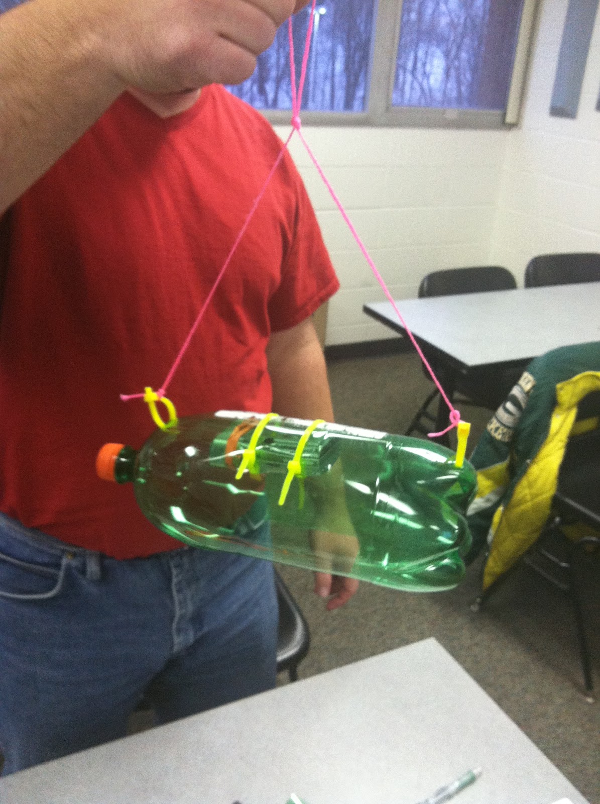
Figure 3: 2 liter design. Camera is fastened with zip ties. A lense window is cut out of the bottom of the bottle.

Figure 4: For the multi-shot function to work the shutter button must remain depressed.

 

The second low altitude balloon uses a free floating camera design housed in the top half of a vinegar jug (Figure 5).  The advantage of this design is it lets the camera behave independently of the balloon.  Ideally the images will be taken as near to vertical as possible to allow for better image interpretation.  However, wind gusts may cause the camera to begin to swing creating varying oblique’s making the process of mosaicking difficult.

Figure 5: Free floating camera design.

 

It should be noted that these designs are only in their preliminary stages.  They are likely to be modified and tested rigorously prior to launch.                   

High Altitude Balloon:

For this project the HABL design was primarily where I focused my work.  Similar to the low altitude balloon, all resources used in its construction needed to be recorded and weighed.  However, with the HABL the return trip also has to be accounted for.  A five foot parachute is being used to safely transport our payload box back to the earth’s surface (figure 6).  Knowing the size of this parachute places certain limitations to the payload that can added.  If the box contains too much material we run the risk of having a dangerous descent speed.  We began testing our parachute with various weights to record descent speed (figure 7).

Figure 6: A 5 foot parachute will be used to safely return our payload box.

                           Figure 7: Testing our parachute with an approximate payload of 2 pounds

For retrieving the balloon a GPS tracker must also be included. With roughly estimate the balloon to travel up to 80 miles away from the launch site.

Deciding upon the total weight of our payload was quite difficult.  Every piece of string, rubber band, and insulation had to be recorded to ensure an accurate total.  It didn’t take long to have over two pounds of material including the camera, heating packs, rope, and the GPS.  Using this estimate, it was decided that our balloon must be able to handle 2-4lbs.

While constructing the rig, the temperatures of our electronics must also be controlled.  If the temperatures fall too low within our payload box we run the risk of losing battery power to our equipment.  To keep things warm at 95,000 feet our payload box needs to be sealed, insulated, and supplied with heating packs.  However, this adds another complexity to our project.  The lack of oxygen in that high of an altitude may have a negative effect on our heat pack’s required chemical reaction.  Our current design uses a minnow bucket payload box with additional insulation (figure 8).  This first design is going to begin certain stress testing shortly and will be modified accordingly.

Figure 8: Cutting additional insulation to keep the equipment warm and working.

 
Discussion:

As you can see above, this project is only in its preliminary stages. Our various designs have yet to be tested and modified.  For the HABL construction I have a number of ideas to minimize weight. One of them being the use of a piece of heat blanket to substitute additional insulation. This could possibly keep the weight down as well as provide further reflectance of heat waves.  Another idea I have for future development is using spray insulations.  The benefit of this is all of the components would not require further securing in place.  Additional holes could be cut into the styrofoam so that power buttons may be depressed.  Further testing on spary insulation will be done to determine how much added weight it may cause. 

Conclusion:

Now that we have a general idea of our balloon designs we can continue our preparation paying more attention to the details. Certain factors that may seem small are often what cause the most problems in the field.  Things such as which knots to use and the best techniques for fastening our components together need more consideration.  Pending test results we will continue improving on or possibly redesigning our constructions. 
 

Exercise 1 Part 2

Introduction:

In part two of exercise one, we revisited our previous terrain model to correct any problems, and create a continuous surface using our data points.  It was determined a re-survey was required to attain more accurate results.  Our group decided to increase the detail of our model by using smaller units of measurement.  The previous 6 inch cells were changed to 8 cm allowing for better interpretation of our data. The methods of this report move from data collection to interpretation of the data.

Above is the sand table model we created. The top left feature seen is a volcano and a stream to the east. A large ridge extends across the western portion of the box.  The chunk of snow seen on the left was difficult to model accurately because of its hard edges and how the interpolation techniques work. (NOTE: this picture was not taken from the origin of our data)

 

Methods:

Similar to part one we recreated a Cartesian coordinate system using grid cells with unique X and Y values. Each cell measured 8 X 8 centimeters providing a sample size of 364 elevation (Z) points. 

The process of measuring the cells, each one measuring 8 square centimeters.

 

After the data is collected in the field, it needs to be manipulated so that X, Y, and Z values are the same units of measurement.  If the X and Y values are not also recorded in centimeter measurements on the spreadsheet, you will have unintentional vertical exaggeration once imported into ArcScene.  When the values were entered into excel the origin was also accidentally changed.  This was fixed by flipping the X values for each row.

By multiply the X and Y values by 8 any vertical exaggeration will be removed since all values are the same units (centimeters).  Below is a revised spreadsheet that is ready to be imported into the ArcMap software for further analysis.

                                                           

Now that all of the data is in the proper format, it can be imported into ArcMap.  This is a simple process of adding the table into the software and displaying the XY data. Once this is done, it will be displayed similar to the image below

The bulk of this project involves using various interpolation methods in analyzing the data in a continuous surface raster.  Five interpolation techniques were used in this process: Inverse Distance Weighted (IDW), Natural Neighbor, Kriging, Spline, and TIN. Following each explanation of the method an image is provided.

Inverse Distance Weighted interpolation calculates values between data points by weighting them according to their distance from the known points. Data points provided decrease in influence as they move further from a particular data point. Below is an image provide by ArcMap describing this method.

The yellow point in this image is created using an algorithm averaging the points surrounding them according to their distance. The greater the distance from this point, the less influence it has on new values. The image below shows how this technique estimates new values to provide a continuous elevation profile of our data.

Using IDW interpolation various features are distinguishable; however, the data points are still visible.

              

The next technique used to calculate a continuous surface is called Natural Neighbor.  Natural Neighbor interpolation uses adjacent data points to construct new values similar to IDW. Below is the data portrayed using this interpolation method.

Similiar to IDW interpolation, all of the features using Natural Neighbors are distinguishable. The image also appears much more smooth, showing a continuous elevation surface. Our river, shown in green, doesn't quite connect; however, as in the real world, river bottom surfaces also fluctuate.

Some of the interpolation tools are very difficult to explain. They use complex algorithms to estimate values not provided. Below is ESRI's explanation of Kriging interpolation.

Kriging is an advanced geostatistical procedure that generates an estimated surface from a scattered set of points with z-values. Unlike other interpolation methods in the Interpolation toolset, to use the Kriging tool effectively involves an interactive investigation of the spatial behavior of the phenomenon represented by the z-values before you select the best estimation method for generating the output surface. (ESRI)

The image below is our data having undergone kriging interpolation. Note the depression found at the top of our volcano in the south east is not present. This was taken into consideration for choosing the best method to represent our data.

Kriging provided a relatively continuous surface; although, it did not represent our model as well as IDW or Natural Neighbor.

 

Spline interpolation created the most accurate representation of our model. The elevation data appears to be very smooth compared to the other methods. The river found in the western portion of our model as well as the volcano is defined quite nicely.  Having additional data points would create an even more accurate depiction of our model’s surface.

The Spline tool uses an interpolation method that estimates values using a mathematical function that minimizes overall surface curvature, resulting in a smooth surface that passes exactly through the input points. (ESRI)

Spline interpolation provided both the most aesthetic as well as accurate depiction of our sand table model.

                                                         

A TIN (Triangular Irregular Networks) surface is created by connecting three data points to one another so that they do not overlap. Since the data points are evenly dispersed across the model, each triangle has the same area. This method provided the least aesthetic depiction of our continuous surface model.

                                                           

After using the different interpolation tools, the surface models are ready to be imported into ArcScene to be spatially examined in three dimensions. Each raster image is added to the program and selected to float on a custom surface. This creates a three dimensional model of our sandtable.
Below is the finalized product produced using the various interpolation methods of our data. (NOTE: None of the three dimensional images were given any vertical exaggeration.)

Inverse Distance Weighted interpolation created a surface model that made our features distinguishable; however, they were not as continuous as the other methods.

The Natural Neighbor interpolation provided a very accurate three dimensional surface model. It was very similar in appearance as the Spline model.

Kriging interpolation provided the least accurate results of our data. The stream and the volcano depression are hardly noticable.

Spline interpolation turned out very similar to Natural Neighbor. It provided the most continuous as well as the most accurate model of our sand table. All terrain features are clearly distinguishable.

Discussion:

As stated above, Spline interpolation created the most visually appealing and accurate portrayal of the data provided. The various landform features stand out from the rest and can be easily identified. Provided additional sample points, the digital models would be even more accurate.  If given more time on this project, smaller cells could result in more detailed images throughout the model.

Having the data arranged within a spreadsheet using matching units, also allows for the project to be reexamined in further detail if necessary.  If a certain feature needs to be examined further, one can simply go back to their constructed model, measure the X and Y coordinates, and add more points around the feature.

The final product. Spline interpolation rendered in three dimensions with 30% transparency and a hillshade elevation model underneath.

Conclusion:

This activity provided a great example stressing the importance of critical thinking. Each group devised their own plan to construct a digit surface model.  Having finished the project, we are now able to present our findings and learn from each other’s methods.

Although we used small models to portray features of earth’s surface, this technique still applies when examining a larger area.  Technique’s such as this can be used in field research with the minimum amount of technology.  Various aspects of this research will likely be encountered in my future as a geospatial analyst.

Creating a Digital Elevation Surface

Introduction:

        Technology often fails-- this was an underlying theme presented to us in our first assignment of geog336. In times where technology fails, it is crucial to have the ability to think critically to overcome our reliance on the plethora of gadgets making up our field research arsenal.  Simply put, the most important skill to acquire through higher education is the ability to think critically.

Methods:

  In our first assignment, we were to use improvised survey techniques to create an elevation model in the form of a sand table. Our study area for this assignment was a gardening box measuring roughly 8 x 4 feet.
We began our survey by creating various terrain features such as hills, valleys, depressions, streams, etc.. Sea level was initially defined as being level with the top surface of the 2 x 8's creating the gardening box.  To simplify the process of importing the data into ArcGIS we kept all values positive and chose to change what was considered sea level.
        To record the elevation data we needed to create a method of identifying where each feature was located.  We designed a grid coordinate system with x,y, and z values with cells being 6 x 6 in. Each cell was recorded in relation to the origin on the northeast corner of the box. Once the layout was created we used a tape measure to find and record our elevation data. Measurements were taken from where the ruler touched the terrain surface to where it intersected with our grid.  After our data was recorded we went to the computer lab and entered it into a spread sheet to be imported into a GIS.

 Beatriz and Nick measuring our grid 

Discussion:

Having the opportunity to conduct field work in our discipline is very important.  It helps you to realize that things don't always work out as they do on pen and paper.  This emphasizes the importance of being able to think critically in overcoming any dilemmas you encounter.   Going into the project I had an elaborate idea of how I wanted to conduct the survey; however, it didn't turn out exactly as planned.  Instead of using nails to anchor the string for our cells, I figured tape would work fine.  I didn't take into consideration the below zero temperatures would make it difficult for the adhesive to bond.
A concern of mine related to the data gathering process is the amount of error that will likely have occurred.  If elevation values weren't recorded exactly in the center of our cells our results could be thrown off. Also, our cells measuring 6 x 6 inches doesn't allow for very precise data, especially considering we only recorded one elevation per cell. Two ways to alleviate this problem would be to either make smaller cells or to measure in multiple areas in each cell and calculate the mean.  The GIS software has the ability to interpolate new data points; however, you need to provide a large enough sample for it to work well.  During the second phase of this project, it is likely that our data set will have to be altered in a way to make it resemble interval data. As is our data is somewhat confusing since larger numbers actually represent areas of lower elevation.

Above is our data sample. Note: the larger the number the lower the elevation this may present a problem. 

Conclusion:

        This assignment provided a great opportunity to think critically when given the bare minimum of instructions. How we completed the project was left entirely up to us and there were no linear paths to follow. Many classes provide all the instructions from start to finish and, more often than not, the skills you learn are difficult to retain. In the second part of this assignment, we will be Importing our data to see how it spatially turns out. During this process it will be much more clear whether or not our methods were successful.